Introduction to single cell data science

Part 1

Learning objectives

Learn what are genomic data and how are they generated?
What is a GRanges object?
What are some advantages of applying tidy principles to genomic data?
What is a SingleCellExperiment object?

Materials

We will go through the slides available here:

https://docs.google.com/presentation/d/1VFL4OxK44Q7b1c-Vk9PDnroT-R5_aQP2LRfJaHXQedo/edit?usp=sharing

Part 2

Learning objectives

Remind ourselves of basics of tidyverse functions (mostly dplyr and ggplot2).
Introduce how to preprocess data and to perform principal components analysis (PCA), a widely used method for dimensionality reduction.

Palmer penguins

In this section, we give an example of using tidyverse functions with the palmerpenguins dataset available as a CRAN package.

[Source: Artwork by Allison Horst]

library(palmerpenguins) # penguins!
suppressPackageStartupMessages({
  library(ggplot2) # "grammar of graphics" plots
  library(dplyr) # data pliers
})

We can select first three rows and two columns:

penguins |> 
  slice(1:3) |>
  select(species, island)

# A tibble: 3 × 2
  species island   
  <fct>   <fct>    
1 Adelie  Torgersen
2 Adelie  Torgersen
3 Adelie  Torgersen

And estimate the average body mass in grams using summarize():

penguins |> 
  summarize(ave_mass = mean(body_mass_g, na.rm=TRUE))

# A tibble: 1 × 1
  ave_mass
     <dbl>
1    4202.

Rearranging how we omit NA values, we get the same:

penguins |> 
  na.omit() |> 
  summarize(ave_mass = mean(body_mass_g))

# A tibble: 1 × 1
  ave_mass
     <dbl>
1    4207.

Or we can also drop NA values entirely and modify our original dataset

penguins <- penguins |> 
  na.omit()

penguins |> 
  summarize(ave_mass = mean(body_mass_g))

# A tibble: 1 × 1
  ave_mass
     <dbl>
1    4207.

A powerful paradigm is to first group and then summarize:

penguins |> 
  group_by(species, island) |> 
  summarize(ave_mass = mean(body_mass_g))

`summarise()` has grouped output by 'species'. You can override using the
`.groups` argument.

# A tibble: 5 × 3
# Groups:   species [3]
  species   island    ave_mass
  <fct>     <fct>        <dbl>
1 Adelie    Biscoe       3710.
2 Adelie    Dream        3701.
3 Adelie    Torgersen    3709.
4 Chinstrap Dream        3733.
5 Gentoo    Biscoe       5092.

Visualization

These data can also be piped into functions for data visualization:

penguins |> 
  ggplot(aes(species, body_mass_g)) +
  geom_boxplot(aes(fill=species))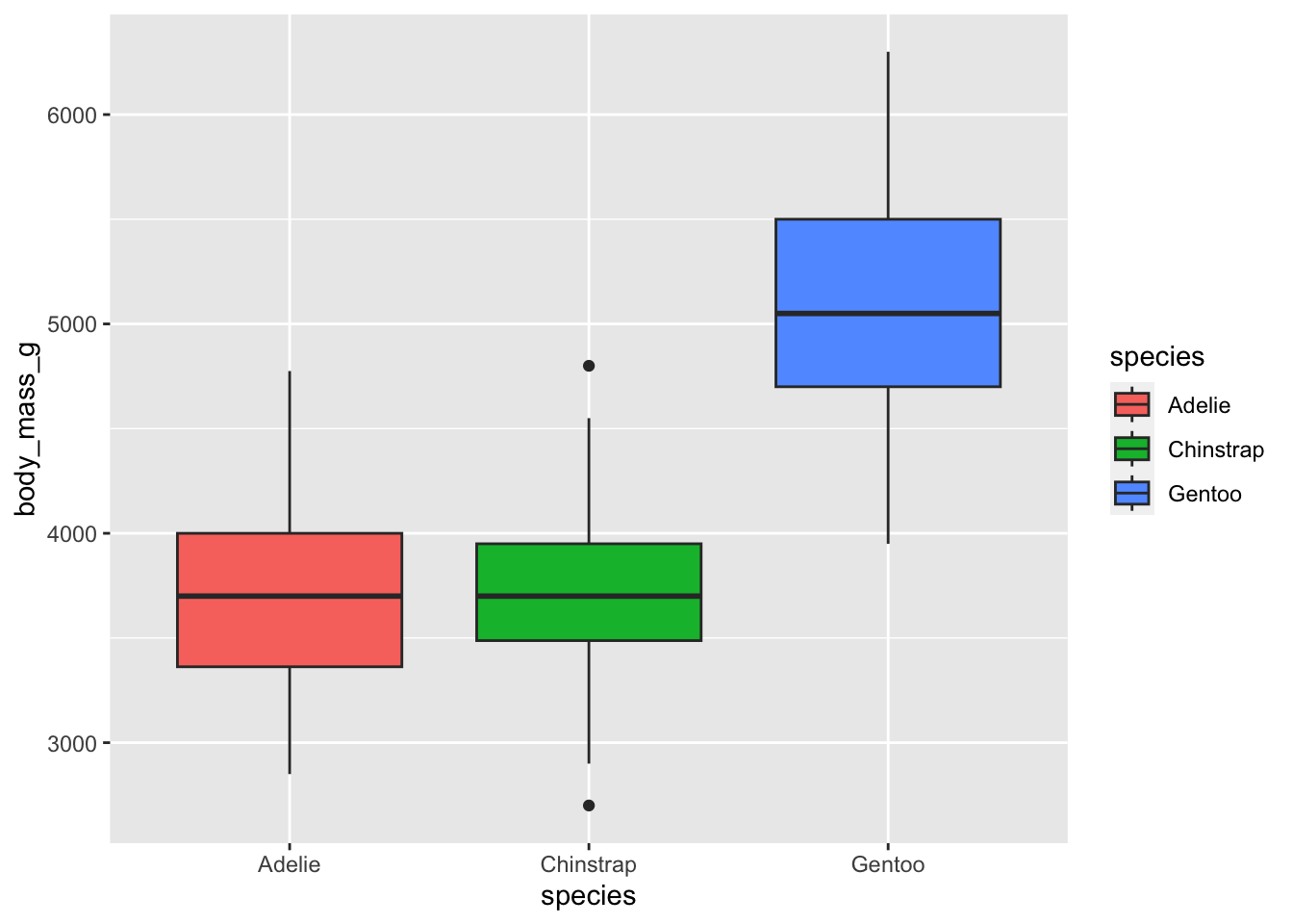

Dimensionality reduction

Next, we will work towards using dimensionality reduction to visualize the penguins in the principal components space.

For the four columns that contain mm or mass, we apply scale(), which centers and scales each variable.

penguins |> 
  mutate(across(contains(c("mm","mass")), scale))

# A tibble: 333 × 8
   species island    bill_length_mm[,1] bill_depth_mm[,1] flipper_length_mm[,1]
   <fct>   <fct>                  <dbl>             <dbl>                 <dbl>
 1 Adelie  Torgersen             -0.895             0.780                -1.42 
 2 Adelie  Torgersen             -0.822             0.119                -1.07 
 3 Adelie  Torgersen             -0.675             0.424                -0.426
 4 Adelie  Torgersen             -1.33              1.08                 -0.568
 5 Adelie  Torgersen             -0.858             1.74                 -0.782
 6 Adelie  Torgersen             -0.931             0.323                -1.42 
 7 Adelie  Torgersen             -0.876             1.24                 -0.426
 8 Adelie  Torgersen             -0.529             0.221                -1.35 
 9 Adelie  Torgersen             -0.986             2.05                 -0.711
10 Adelie  Torgersen             -1.72              2.00                 -0.212
# ℹ 323 more rows
# ℹ 3 more variables: body_mass_g <dbl[,1]>, sex <fct>, year <int>

Visualizing the scaled data (i.e. y-axis has changed, but distribution is the same).

penguins |> 
  mutate(across(contains(c("mm","mass")), scale)) |> 
  ggplot(aes(species, body_mass_g)) +
  geom_boxplot(aes(fill=species))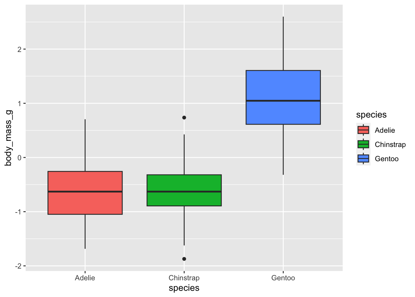

Let’s create a new matrix called scaled with just the four columns scaled.

scaled <- penguins |> 
  select(contains(c("mm","mass"))) |> 
  mutate(across(everything(), scale))
scaled

# A tibble: 333 × 4
   bill_length_mm[,1] bill_depth_mm[,1] flipper_length_mm[,1] body_mass_g[,1]
                <dbl>             <dbl>                 <dbl>           <dbl>
 1             -0.895             0.780                -1.42           -0.568
 2             -0.822             0.119                -1.07           -0.506
 3             -0.675             0.424                -0.426          -1.19 
 4             -1.33              1.08                 -0.568          -0.940
 5             -0.858             1.74                 -0.782          -0.692
 6             -0.931             0.323                -1.42           -0.723
 7             -0.876             1.24                 -0.426           0.581
 8             -0.529             0.221                -1.35           -1.25 
 9             -0.986             2.05                 -0.711          -0.506
10             -1.72              2.00                 -0.212           0.240
# ℹ 323 more rows

Then, we can apply the function prcomp() to calculate the principal components 1 to 4.

Under the hood, the function uses a singular value decomposition of the centered and scaled data matrix (not using eigen on the covariance matrix). Often preferred for numerical accuracy.

scaled |> 
  prcomp()

Standard deviations (1, .., p=4):
[1] 1.6569115 0.8821095 0.6071594 0.3284579

Rotation (n x k) = (4 x 4):
                         PC1         PC2        PC3        PC4
bill_length_mm     0.4537532 -0.60019490 -0.6424951  0.1451695
bill_depth_mm     -0.3990472 -0.79616951  0.4258004 -0.1599044
flipper_length_mm  0.5768250 -0.00578817  0.2360952 -0.7819837
body_mass_g        0.5496747 -0.07646366  0.5917374  0.5846861

Some useful things about output:

pca <- scaled |> 
  prcomp()

names(pca)

[1] "sdev"     "rotation" "center"   "scale"    "x"

dim(pca$x)

[1] 333   4

head(pca$x)

           PC1         PC2         PC3        PC4
[1,] -1.850808 -0.03202119  0.23454869  0.5276026
[2,] -1.314276  0.44286031  0.02742880  0.4011230
[3,] -1.374537  0.16098821 -0.18940423 -0.5278675
[4,] -1.882455  0.01233268  0.62792772 -0.4721826
[5,] -1.917096 -0.81636958  0.69999797 -0.1961213
[6,] -1.770356  0.36567266 -0.02841769  0.5046092

Visualize

penguins |> 
  bind_cols(pca$x) |> 
  ggplot(aes(PC1, PC2, color=species)) + 
  geom_point()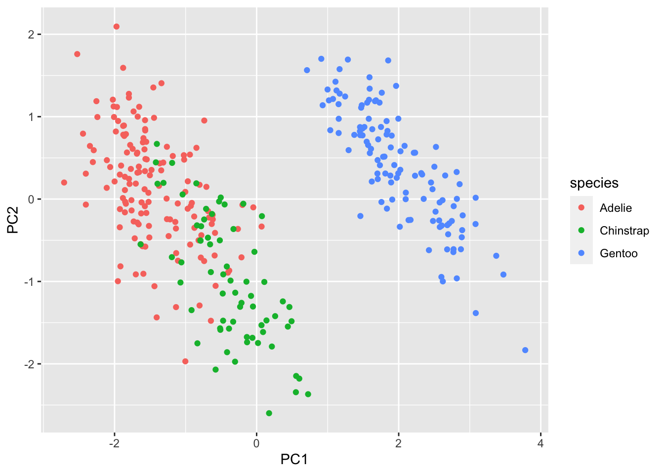

Part 3

In this next section, we move into the analysis of single-cell transcriptomics data with a goal of learning the basic steps for data wrangling these data to calculate top principal components where each point is a cell (instead of a penguin).

Learning objectives

Be able to create a single-cell count matrix and read it into R
Recognize and define the SingleCellExperiment S4 class in R/Bioconductor to store single-cell data
Be able to describe a standard workflow for analyzing single-cell data
Be able to run code for a standard workflow starting from loading a SingleCellExperiment in R and identifying clusters.

Overview

NGS data from scRNA-seq experiments must be converted into a matrix of expression values.

This is usually a count matrix containing the number of reads (or UMIs) mapped to each gene (row) in each cell (column). Once this quantification is complete, we can proceed with our downstream statistical analyses in R.

Constructing a count matrix from raw scRNA-seq data requires some thought as the term “single-cell RNA-seq” encompasses a variety of different experimental protocols.

`SingleCellExperiment` Class

One of the main strengths of the Bioconductor project lies in the use of a common data infrastructure that powers interoperability across packages.

Users should be able to analyze their data using functions from different Bioconductor packages without the need to convert between formats.

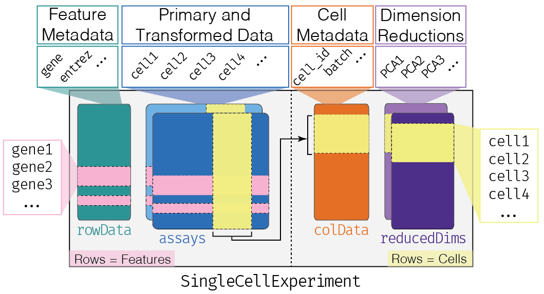
To this end, the SingleCellExperiment class (from the SingleCellExperiment package) serves as the common currency for data exchange across 70+ single-cell-related Bioconductor packages.

This class implements a data structure that stores all aspects of our single-cell data - gene-by-cell expression data, per-cell metadata and per-gene annotation - and manipulate them in a synchronized manner.

[source]

Each piece of (meta)data in the SingleCellExperiment is represented by a separate “slot”.

(This terminology comes from the S4 class system, but that’s not important right now).

If we imagine the SingleCellExperiment object to be a cargo ship, the slots can be thought of as individual cargo boxes with different contents, e.g., certain slots expect numeric matrices whereas others may expect data frames.

If you want to know more about the available slots, their expected formats, and how we can interact with them, check out this chapter.

`SingleCellExperiment` Example

Let’s show you what a SingleCellExperiment (or sce for short) looks like.

sce

class: SingleCellExperiment 
dim: 20006 3005 
metadata(0):
assays(1): counts
rownames(20006): Tspan12 Tshz1 ... mt-Rnr1 mt-Nd4l
rowData names(1): featureType
colnames(3005): 1772071015_C02 1772071017_G12 ... 1772066098_A12
  1772058148_F03
colData names(10): tissue group # ... level1class level2class
reducedDimNames(0):
mainExpName: endogenous
altExpNames(2): ERCC repeat

This SingleCellExperiment object has 20006 genes and 3005 cells.

We can pull out the counts matrix with the counts() function and the corresponding rowData() and colData():

counts(sce)[1:5, 1:5]

         1772071015_C02 1772071017_G12 1772071017_A05 1772071014_B06
Tspan12               0              0              0              3
Tshz1                 3              1              0              2
Fnbp1l                3              1              6              4
Adamts15              0              0              0              0
Cldn12                1              1              1              0
         1772067065_H06
Tspan12               0
Tshz1                 2
Fnbp1l                1
Adamts15              0
Cldn12                0

rowData(sce)

DataFrame with 20006 rows and 1 column
         featureType
         <character>
Tspan12   endogenous
Tshz1     endogenous
Fnbp1l    endogenous
Adamts15  endogenous
Cldn12    endogenous
...              ...
mt-Co2          mito
mt-Co1          mito
mt-Rnr2         mito
mt-Rnr1         mito
mt-Nd4l         mito

colData(sce)

DataFrame with 3005 rows and 10 columns
                       tissue   group # total mRNA mol      well       sex
                  <character> <numeric>      <numeric> <numeric> <numeric>
1772071015_C02       sscortex         1           1221         3         3
1772071017_G12       sscortex         1           1231        95         1
1772071017_A05       sscortex         1           1652        27         1
1772071014_B06       sscortex         1           1696        37         3
1772067065_H06       sscortex         1           1219        43         3
...                       ...       ...            ...       ...       ...
1772067059_B04 ca1hippocampus         9           1997        19         1
1772066097_D04 ca1hippocampus         9           1415        21         1
1772063068_D01       sscortex         9           1876        34         3
1772066098_A12 ca1hippocampus         9           1546        88         1
1772058148_F03       sscortex         9           1970        15         3
                     age  diameter        cell_id       level1class level2class
               <numeric> <numeric>    <character>       <character> <character>
1772071015_C02         2         1 1772071015_C02      interneurons       Int10
1772071017_G12         1       353 1772071017_G12      interneurons       Int10
1772071017_A05         1        13 1772071017_A05      interneurons        Int6
1772071014_B06         2        19 1772071014_B06      interneurons       Int10
1772067065_H06         6        12 1772067065_H06      interneurons        Int9
...                  ...       ...            ...               ...         ...
1772067059_B04         4       382 1772067059_B04 endothelial-mural       Peric
1772066097_D04         7        12 1772066097_D04 endothelial-mural        Vsmc
1772063068_D01         7       268 1772063068_D01 endothelial-mural        Vsmc
1772066098_A12         7       324 1772066098_A12 endothelial-mural        Vsmc
1772058148_F03         7         6 1772058148_F03 endothelial-mural        Vsmc

A typical single-cell workflow

Here, we provide an overview of the framework of a typical scRNA-seq analysis workflow:

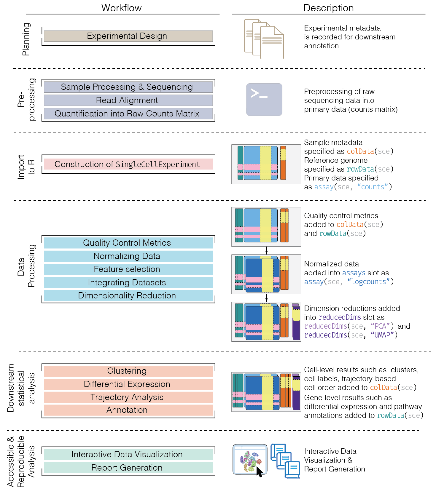
In the simplest case, the workflow has the following form:

We compute quality control metrics to remove low-quality cells that would interfere with downstream analyses. These cells may have been damaged during processing or may not have been fully captured by the sequencing protocol. Common metrics includes the total counts per cell, the proportion of spike-in or mitochondrial reads and the number of detected features.
We convert the counts into normalized expression values to eliminate cell-specific biases (e.g., in capture efficiency). This allows us to perform explicit comparisons across cells in downstream steps like clustering. We also apply a transformation, typically log, to adjust for the mean-variance relationship.
We perform feature selection to pick a subset of interesting features for downstream analysis. This is done by modelling the variance across cells for each gene and retaining genes that are highly variable. The aim is to reduce computational overhead and noise from uninteresting genes.
We apply dimensionality reduction to compact the data and further reduce noise. Principal components analysis is typically used to obtain an initial low-rank representation for more computational work, followed by more aggressive methods like \(t\)-stochastic neighbor embedding for visualization purposes.
We cluster cells into groups according to similarities in their (normalized) expression profiles. This aims to obtain groupings that serve as empirical proxies for distinct biological states. We typically interpret these groupings by identifying differentially expressed marker genes between clusters.

Quick start (simple)

Here, we use the a droplet-based retina dataset from Macosko et al. (2015), provided in the scRNAseq package. This starts from a count matrix and finishes with clusters in preparation for biological interpretation. We also demonstrate how to identify differentially expressed genes between the clusters.

library(scRNAseq)
sce <- MacoskoRetinaData()

see ?scRNAseq and browseVignettes('scRNAseq') for documentation

loading from cache

see ?scRNAseq and browseVignettes('scRNAseq') for documentation

loading from cache

# Quality control (using mitochondrial genes).
library(scater)

Loading required package: scuttle

is.mito <- grepl("^MT-", rownames(sce)) # find mitochondrial genes
qcstats <- perCellQCMetrics(sce, subsets=list(Mito=is.mito)) # calculate QC metrics 
filtered <- quickPerCellQC(qcstats, percent_subsets="subsets_Mito_percent") # filter base on QC metrics
sce <- sce[, !filtered$discard] # subset object for post-QC analyses

# Normalization.
sce <- logNormCounts(sce)

# Feature selection (which genes are most important)? 
library(scran)
dec.retina <- modelGeneVar(sce)
hvg <- getTopHVGs(dec.retina, prop=0.1)

# Visualizing the fit:
fit.retina <- metadata(dec.retina)
plot(fit.retina$mean, fit.retina$var, xlab="Mean of log-expression",
    ylab="Variance of log-expression")
curve(fit.retina$trend(x), col="dodgerblue", add=TRUE, lwd=2)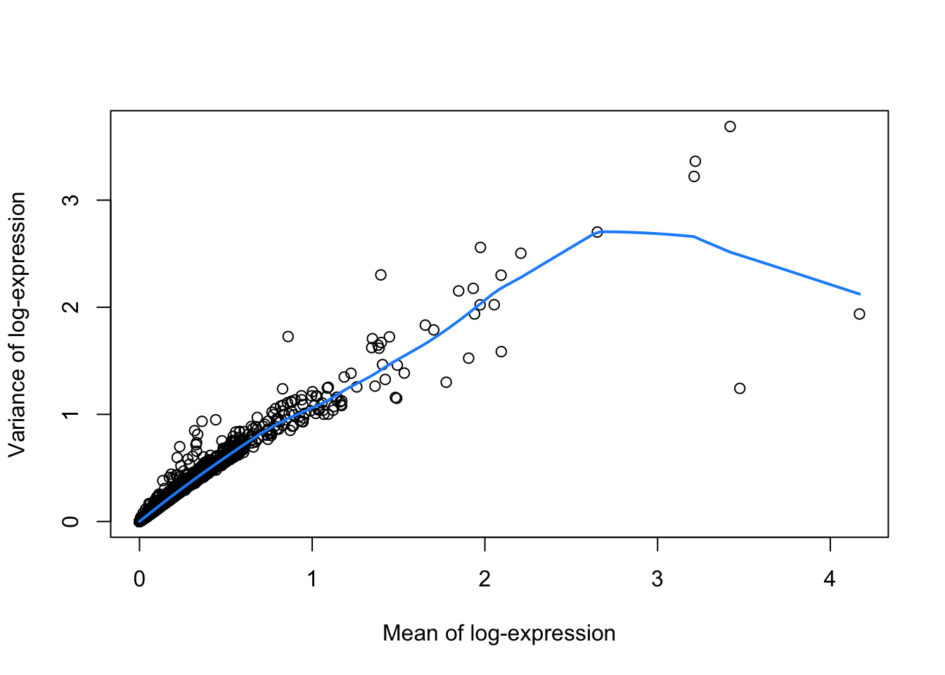

# PCA
library(scater)
set.seed(1234)
sce <- runPCA(sce, ncomponents=25, subset_row=hvg)

# Clustering.
library(bluster)
colLabels(sce) <- clusterCells(sce, use.dimred='PCA',
    BLUSPARAM=NNGraphParam(cluster.fun="louvain"))

# Visualization of PC1 vs PC2
plotPCA(sce, colour_by="label")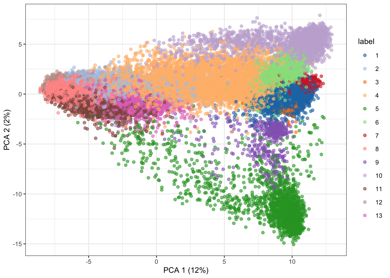

# UMAP visualization 
sce <- runUMAP(sce, dimred = 'PCA')
plotUMAP(sce, colour_by="label")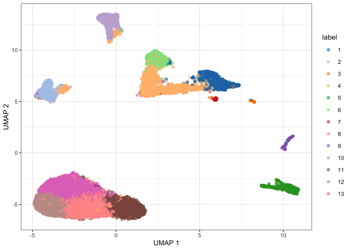

UMAP plot of the retina dataset, where each point is a cell and is colored by the assigned cluster identity.

For more information

If you could like to know more, check out this book:

https://bioconductor.org/books/release/OSCA/

Part 4

Last, we will briefly highlight the tidySingleCellExperiment package (https://www.bioconductor.org/packages/SingleCellExperiment) that allows you to leverage functions from dplyr, tidyr, and ggplot2 with a SingleCellExperiment object.

This package is part of a large set of packages called tidyomics, which bridges the two worlds of tidy principles in R with Bioconductor.

It is similar to tidyverse in that it installs a series of packages that are designed to work with different types of objects in Bioconductor. Specifically, it installs:

plyranges = for data with GRanges
tidybulk = for bulk RNA-sequencing data
tidySummarizedExperiment = for data in a SummarizedExperiment object
tidySingleCellExperiment = for data in a SingleCellExperiment object
tidySpatialExperiment = for data in a SpatialExperiment object
tidyseurat = to bring Seurat to the tidyverse
nullranges = to generate of sets of GRranges representing the null hypothesis

For more information:

manuscript: https://doi.org/10.1101/2023.09.10.557072
to install tidyomics: https://github.com/tidyomics/tidyomics

remotes::install_github("tidyomics/tidyomics")

Overview

suppressPackageStartupMessages({
  library(tidySummarizedExperiment) # allow dplyr
})

sce |>
  addPerCellQC(subsets=list(Mito=is.mito)) |>
  colData()

DataFrame with 45877 rows and 10 columns
                        cell.id   cluster sizeFactor    label       sum
                    <character> <integer>  <numeric> <factor> <numeric>
r1_GGCCGCAGTCCG r1_GGCCGCAGTCCG         2    28.0131        1     37487
r1_CTTGTGCGGGAA r1_CTTGTGCGGGAA         2    23.9479        1     32047
r1_GCGCAACTGCTC r1_GCGCAACTGCTC         2    21.0343        1     28148
r1_GATTGGGAGGCA r1_GATTGGGAGGCA         2    15.2197        1     20367
r1_CCTCCTAGTTGG r1_CCTCCTAGTTGG        NA    14.6167        1     19560
...                         ...       ...        ...      ...       ...
p1_TCAAAAGCCGGG p1_TCAAAAGCCGGG        24   0.610523       13       817
p1_ATTAAGTTCCAA p1_ATTAAGTTCCAA        34   0.610523       5        817
p1_CTGTCTGAGACC p1_CTGTCTGAGACC         2   0.610523       1        817
p1_TAACGCGCTCCT p1_TAACGCGCTCCT        24   0.609776       11       816
p1_ATTCTTGTTCTT p1_ATTCTTGTTCTT        24   0.609776       8        816
                 detected subsets_Mito_sum subsets_Mito_detected
                <integer>        <numeric>             <integer>
r1_GGCCGCAGTCCG      7243              427                    14
r1_CTTGTGCGGGAA      6933              503                    15
r1_GCGCAACTGCTC      6397              460                    13
r1_GATTGGGAGGCA      5740              326                    11
r1_CCTCCTAGTTGG      5779              264                     9
...                   ...              ...                   ...
p1_TCAAAAGCCGGG       537               13                     4
p1_ATTAAGTTCCAA       574               10                     5
p1_CTGTCTGAGACC       637               24                     7
p1_TAACGCGCTCCT       488               27                     5
p1_ATTCTTGTTCTT       484               16                     4
                subsets_Mito_percent     total
                           <numeric> <numeric>
r1_GGCCGCAGTCCG              1.13906     37487
r1_CTTGTGCGGGAA              1.56957     32047
r1_GCGCAACTGCTC              1.63422     28148
r1_GATTGGGAGGCA              1.60063     20367
r1_CCTCCTAGTTGG              1.34969     19560
...                              ...       ...
p1_TCAAAAGCCGGG              1.59119       817
p1_ATTAAGTTCCAA              1.22399       817
p1_CTGTCTGAGACC              2.93758       817
p1_TAACGCGCTCCT              3.30882       816
p1_ATTCTTGTTCTT              1.96078       816

# Identify variable genes with scran
variable_genes <-
    sce %>%
    modelGeneVar() %>%
    getTopHVGs(prop=0.1)

# Perform PCA with scater
retina_pca <-
    sce %>%
    runPCA(subset_row=variable_genes)

plotPCA(retina_pca, colour_by="label")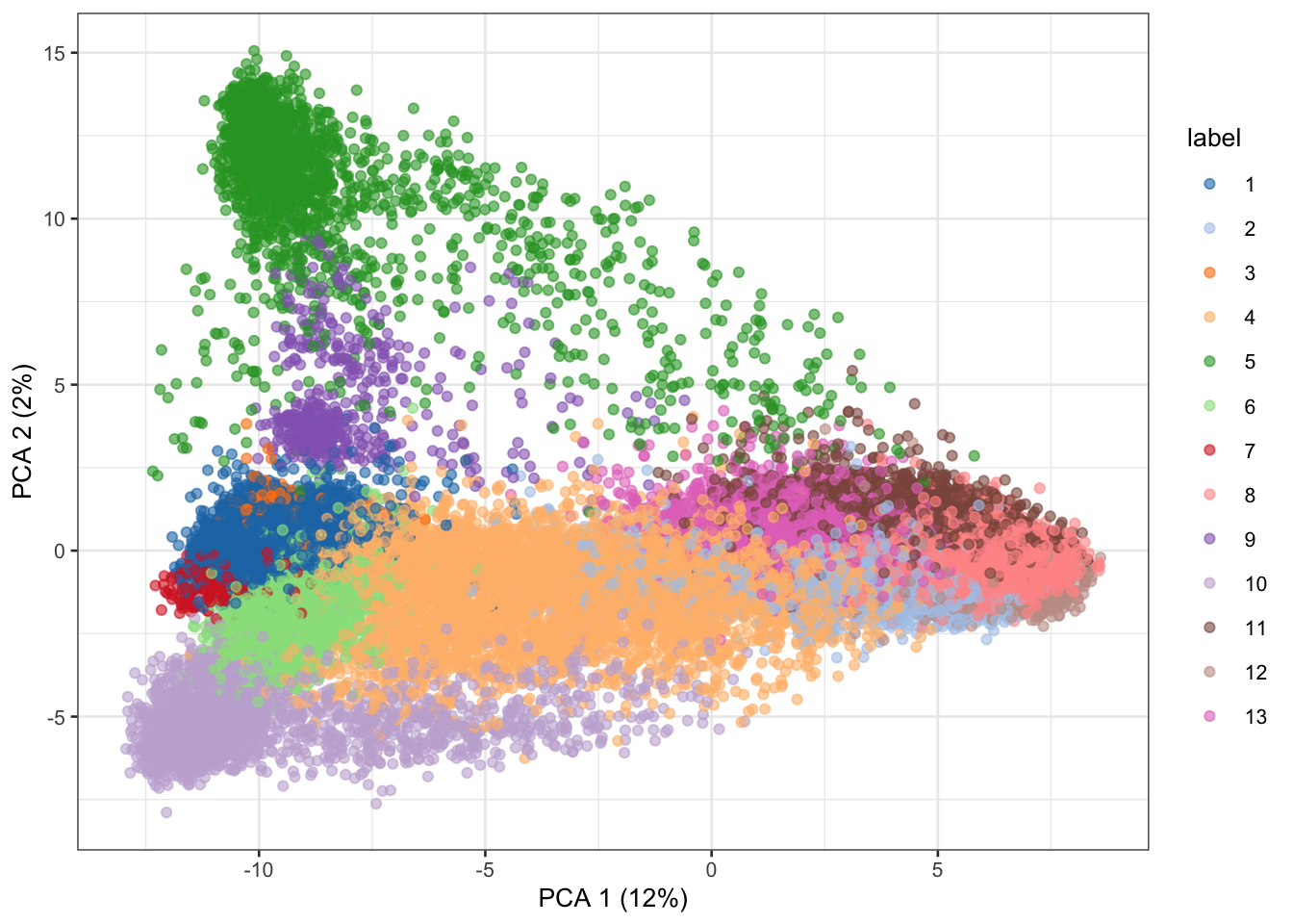

Session Info

sessionInfo()

R version 4.3.1 (2023-06-16)
Platform: aarch64-apple-darwin20 (64-bit)
Running under: macOS Ventura 13.4.1

Matrix products: default
BLAS:   /Library/Frameworks/R.framework/Versions/4.3-arm64/Resources/lib/libRblas.0.dylib 
LAPACK: /Library/Frameworks/R.framework/Versions/4.3-arm64/Resources/lib/libRlapack.dylib;  LAPACK version 3.11.0

locale:
[1] en_US.UTF-8/en_US.UTF-8/en_US.UTF-8/C/en_US.UTF-8/en_US.UTF-8

time zone: America/New_York
tzcode source: internal

attached base packages:
[1] stats4    stats     graphics  grDevices utils     datasets  methods  
[8] base     

other attached packages:
 [1] tidySummarizedExperiment_1.10.0 bluster_1.10.0                 
 [3] scran_1.28.2                    scater_1.28.0                  
 [5] scuttle_1.9.4                   scRNAseq_2.14.0                
 [7] SingleCellExperiment_1.22.0     SummarizedExperiment_1.30.2    
 [9] Biobase_2.60.0                  GenomicRanges_1.52.0           
[11] GenomeInfoDb_1.36.3             IRanges_2.34.1                 
[13] S4Vectors_0.38.1                BiocGenerics_0.46.0            
[15] MatrixGenerics_1.12.3           matrixStats_1.0.0              
[17] dplyr_1.1.3                     ggplot2_3.4.3                  
[19] palmerpenguins_0.1.1           

loaded via a namespace (and not attached):
  [1] rstudioapi_0.15.0             jsonlite_1.8.7               
  [3] magrittr_2.0.3                ggbeeswarm_0.7.2             
  [5] GenomicFeatures_1.52.2        farver_2.1.1                 
  [7] rmarkdown_2.24                BiocIO_1.10.0                
  [9] zlibbioc_1.46.0               vctrs_0.6.3                  
 [11] memoise_2.0.1                 Rsamtools_2.16.0             
 [13] DelayedMatrixStats_1.22.6     RCurl_1.98-1.12              
 [15] htmltools_0.5.6               S4Arrays_1.0.6               
 [17] progress_1.2.2                AnnotationHub_3.8.0          
 [19] curl_5.0.2                    BiocNeighbors_1.18.0         
 [21] htmlwidgets_1.6.2             plotly_4.10.2                
 [23] cachem_1.0.8                  GenomicAlignments_1.36.0     
 [25] igraph_1.5.1                  mime_0.12                    
 [27] lifecycle_1.0.3               pkgconfig_2.0.3              
 [29] rsvd_1.0.5                    Matrix_1.6-1                 
 [31] R6_2.5.1                      fastmap_1.1.1                
 [33] GenomeInfoDbData_1.2.10       shiny_1.7.5                  
 [35] digest_0.6.33                 colorspace_2.1-0             
 [37] AnnotationDbi_1.62.2          dqrng_0.3.1                  
 [39] irlba_2.3.5.1                 ExperimentHub_2.8.1          
 [41] RSQLite_2.3.1                 beachmat_2.16.0              
 [43] filelock_1.0.2                labeling_0.4.3               
 [45] fansi_1.0.4                   httr_1.4.7                   
 [47] abind_1.4-5                   compiler_4.3.1               
 [49] bit64_4.0.5                   withr_2.5.0                  
 [51] BiocParallel_1.34.2           viridis_0.6.4                
 [53] DBI_1.1.3                     biomaRt_2.56.1               
 [55] rappdirs_0.3.3                DelayedArray_0.26.7          
 [57] rjson_0.2.21                  tools_4.3.1                  
 [59] vipor_0.4.5                   beeswarm_0.4.0               
 [61] interactiveDisplayBase_1.38.0 httpuv_1.6.11                
 [63] glue_1.6.2                    restfulr_0.0.15              
 [65] promises_1.2.1                grid_4.3.1                   
 [67] cluster_2.1.4                 generics_0.1.3               
 [69] gtable_0.3.4                  tidyr_1.3.0                  
 [71] ensembldb_2.24.0              data.table_1.14.8            
 [73] hms_1.1.3                     metapod_1.7.0                
 [75] BiocSingular_1.16.0           ScaledMatrix_1.8.1           
 [77] xml2_1.3.5                    utf8_1.2.3                   
 [79] XVector_0.40.0                RcppAnnoy_0.0.21             
 [81] ggrepel_0.9.3                 BiocVersion_3.17.1           
 [83] pillar_1.9.0                  stringr_1.5.0                
 [85] limma_3.56.2                  later_1.3.1                  
 [87] BiocFileCache_2.8.0           lattice_0.21-8               
 [89] rtracklayer_1.60.1            bit_4.0.5                    
 [91] tidyselect_1.2.0              locfit_1.5-9.8               
 [93] Biostrings_2.68.1             knitr_1.44                   
 [95] gridExtra_2.3                 ProtGenerics_1.32.0          
 [97] edgeR_3.42.4                  xfun_0.40                    
 [99] statmod_1.5.0                 stringi_1.7.12               
[101] lazyeval_0.2.2                yaml_2.3.7                   
[103] evaluate_0.21                 codetools_0.2-19             
[105] tibble_3.2.1                  BiocManager_1.30.22          
[107] cli_3.6.1                     uwot_0.1.16                  
[109] xtable_1.8-4                  munsell_0.5.0                
[111] Rcpp_1.0.11                   dbplyr_2.3.3                 
[113] png_0.1-8                     XML_3.99-0.14                
[115] parallel_4.3.1                ellipsis_0.3.2               
[117] blob_1.2.4                    prettyunits_1.1.1            
[119] AnnotationFilter_1.24.0       sparseMatrixStats_1.12.2     
[121] bitops_1.0-7                  viridisLite_0.4.2            
[123] scales_1.2.1                  purrr_1.0.2                  
[125] crayon_1.5.2                  rlang_1.1.1                  
[127] KEGGREST_1.40.0

Part 1

Learning objectives

Materials

Part 2

Learning objectives

Palmer penguins

Visualization

Dimensionality reduction

Part 3

Learning objectives

Overview

SingleCellExperiment Class

SingleCellExperiment Example

A typical single-cell workflow

Quick start (simple)

For more information

Part 4

Overview

Session Info

`SingleCellExperiment` Class

`SingleCellExperiment` Example