Pre-lecture materials

Read ahead

Before class, you can prepare by reading the following materials:

https://r4ds.had.co.nz/dates-and-times

Acknowledgements

Material for this lecture was borrowed and adopted from

Learning objectives

At the end of this lesson you will:

Recognize the Date, POSIXct and POSIXlt class types in R to represent dates and times
Learn how to create date and time objects in R using functions from the lubridate package
Learn how dealing with time zones can be frustrating 🙀 but hopefully less so after today’s lecture 😺
Learn how to perform arithmetic operations on dates and times
Learn how plotting systems in R “know” about dates and times to appropriately handle axis labels

Introduction

In this lesson, we will learn how to work with dates and times in R. These may seem simple as you use them all of the time in your day-to-day life, but the more you work with them, the more complicated they seem to get.

Dates and times are hard to work with because they have to reconcile two physical phenomena

The rotation of the Earth and its orbit around the sun AND
A whole raft of geopolitical phenomena including months, time zones, and daylight savings time (DST)

This lesson will not teach you every last detail about dates and times, but it will give you a solid grounding of practical skills that will help you with common data analysis challenges.

Classes for dates and times in R

R has developed a special representation of dates and times

Dates are represented by the Date class
Times are represented by the POSIXct or the POSIXlt class

Important point in time

Dates are stored internally as the number of days since 1970-01-01
Times are stored internally as the number of seconds since 1970-01-01

In computing, Unix time (also known as Epoch time, Posix time, seconds since the Epoch, Unix timestamp, or UNIX Epoch time) is a system for describing a point in time.

It is the number of seconds that have elapsed since the Unix epoch, excluding leap seconds. The Unix epoch is 00:00:00 UTC on 1 January 1970.

Unix time originally appeared as the system time of Unix, but is now used widely in computing, for example by filesystems; some Python language library functions handle Unix time.[4]

https://en.wikipedia.org/wiki/Unix_time

The `lubridate` package

Here, we will focus on the lubridate R package, which makes it easier to work with dates and times in R.

Pro-tip

Check out the lubridate cheat sheet at https://lubridate.tidyverse.org

A few things to note about it:

It largely replaces the default date/time functions in base R
It contains methods for date/time arithmetic
It handles time zones, leap year, leap seconds, etc.

[Source: Artwork by Allison Horst]

lubridate is installed when you install tidyverse, but it is not loaded when you load tidyverse. Alternatively, you can install it separately.

install.packages("lubridate")

library(tidyverse)
library(lubridate)

Creating date/times

There are three types of date/time data that refer to an instant in time:

A date. Tibbles print this as <date>.
A time within a day. Tibbles print this as <time>.
A date-time is a date plus a time: it uniquely identifies an instant in time (typically to the nearest second). Tibbles print this as <dttm>. Elsewhere in R these are called POSIXct.

Note

We will focus on dates and date-times as R does not have a native class for storing times.

If you to work with only times, you can use the hms package.

You should always use the simplest possible data type that works for your needs.

That means if you can use a date instead of a date-time, you should.

Date-times are substantially more complicated because of the need to handle time zones, which we will come back to at the end of the lesson.

To get the current date or date-time you can use today() or now() from lubridate:

today()

[1] "2022-10-02"

now()

[1] "2022-10-02 23:58:38 EDT"

Otherwise, there are three ways you are likely to create a date/time:

Typical ways to create a date/time in R

From a string
From individual date-time components
From an existing date/time object

They work as follows.

1. From a string

Dates are of the Date class.

x <- today()
class(x)

[1] "Date"

Dates can be coerced from a character strings using some helper functions from lubridate. They automatically work out the format once you specify the order of the component.

To use the helper functions, identify the order in which year, month, and day appear in your dates, then arrange “y”, “m”, and “d” in the same order.

That gives you the name of the lubridate function that will parse your date. For example:

ymd("1970-01-01")

[1] "1970-01-01"

ymd("2017-01-31")

[1] "2017-01-31"

mdy("January 31st, 2017")

[1] "2017-01-31"

dmy("31-Jan-2017")

[1] "2017-01-31"

Pro-tip

When reading in data with read_csv(), you may need to read in as character first and then convert to date/time
Date objects have their own special print() methods that will always format as “YYYY-MM-DD”
These functions also take unquoted numbers.

ymd(20170131)

[1] "2017-01-31"

Alternate Formulations

Different locales have different ways of formatting dates

ymd("2016-09-13")  ## International standard

[1] "2016-09-13"

ymd("2016/09/13")  ## Just figure it out

[1] "2016-09-13"

mdy("09-13-2016")  ## Mostly U.S.

[1] "2016-09-13"

dmy("13-09-2016")  ## Europe

[1] "2016-09-13"

All of the above are valid and lead to the exact same object.

Even if the individual dates are formatted differently, ymd() can usually figure it out.

x <- c("2016-04-05", 
       "2016/05/06",
       "2016,10,4")
ymd(x)

[1] "2016-04-05" "2016-05-06" "2016-10-04"

Cool right?

2. From individual date-time components

Sometimes the date components will come across multiple columns in a dataset.

library(nycflights13)

flights %>% 
  select(year, month, day)

# A tibble: 336,776 × 3
    year month   day
   <int> <int> <int>
 1  2013     1     1
 2  2013     1     1
 3  2013     1     1
 4  2013     1     1
 5  2013     1     1
 6  2013     1     1
 7  2013     1     1
 8  2013     1     1
 9  2013     1     1
10  2013     1     1
# … with 336,766 more rows

To create a date/time from this sort of input, use

make_date(year,month,day) for dates, or
make_datetime(year,month,day,hour,min,sec,tz) for date-times

We combine these functions inside of mutate to add a new column to our dataset:

flights %>% 
  select(year, month, day) %>% 
  mutate(departure = make_date(year, month, day))

# A tibble: 336,776 × 4
    year month   day departure 
   <int> <int> <int> <date>    
 1  2013     1     1 2013-01-01
 2  2013     1     1 2013-01-01
 3  2013     1     1 2013-01-01
 4  2013     1     1 2013-01-01
 5  2013     1     1 2013-01-01
 6  2013     1     1 2013-01-01
 7  2013     1     1 2013-01-01
 8  2013     1     1 2013-01-01
 9  2013     1     1 2013-01-01
10  2013     1     1 2013-01-01
# … with 336,766 more rows

Questions

The flights also contains a hour and minute column.

flights %>% 
  select(year, month, day, hour, minute)

# A tibble: 336,776 × 5
    year month   day  hour minute
   <int> <int> <int> <dbl>  <dbl>
 1  2013     1     1     5     15
 2  2013     1     1     5     29
 3  2013     1     1     5     40
 4  2013     1     1     5     45
 5  2013     1     1     6      0
 6  2013     1     1     5     58
 7  2013     1     1     6      0
 8  2013     1     1     6      0
 9  2013     1     1     6      0
10  2013     1     1     6      0
# … with 336,766 more rows

Let’s use make_datetime() to create a date-time column called departure:

# try it yourself

3. From other types

You may want to switch between a date-time and a date.

That is the job of as_datetime() and as_date():

today()

[1] "2022-10-02"

as_datetime(today())

[1] "2022-10-02 UTC"

now()

[1] "2022-10-02 23:58:39 EDT"

as_date(now())

[1] "2022-10-02"

Date-Times in R

From a string

ymd() and friends create dates.

To create a date-time from a character string, add an underscore and one or more of “h”, “m”, and “s” to the name of the parsing function:

Times can be coerced from a character string with ymd_hms()

ymd_hms("2017-01-31 20:11:59")

[1] "2017-01-31 20:11:59 UTC"

mdy_hm("01/31/2017 08:01")

[1] "2017-01-31 08:01:00 UTC"

You can also force the creation of a date-time from a date by supplying a timezone:

ymd_hms("2016-09-13 14:00:00")

[1] "2016-09-13 14:00:00 UTC"

ymd_hms("2016-09-13 14:00:00", tz = "America/New_York")

[1] "2016-09-13 14:00:00 EDT"

ymd_hms("2016-09-13 14:00:00", tz = "")

[1] "2016-09-13 14:00:00 EDT"

`POSIXct` or the `POSIXlt` class

Let’s get into some hairy details about date-times. Date-times are represented using the POSIXct or the POSIXlt class in R. What are these things?

`POSIXct`

POSIXct is just a very large integer under the hood. It is a useful class when you want to store times in something like a data frame.

Technically, the POSIXct class represents the number of seconds since 1 January 1970. (In case you were wondering, “POSIXct” stands for “Portable Operating System Interface”, calendar time.)

x <- ymd_hm("1970-01-01 01:00")
class(x)

[1] "POSIXct" "POSIXt"

unclass(x)

[1] 3600
attr(,"tzone")
[1] "UTC"

typeof(x)

[1] "double"

attributes(x)

$class
[1] "POSIXct" "POSIXt" 

$tzone
[1] "UTC"

`POSIXlt`

POSIXlt is a list underneath and it stores a bunch of other useful information like the day of the week, day of the year, month, day of the month

y <- as.POSIXlt(x)
y

[1] "1970-01-01 01:00:00 UTC"

typeof(y)

[1] "list"

attributes(y)

$names
[1] "sec"   "min"   "hour"  "mday"  "mon"   "year"  "wday"  "yday"  "isdst"

$class
[1] "POSIXlt" "POSIXt" 

$tzone
[1] "UTC"

Pro-tip

POSIXlts are rare inside the tidyverse. They do crop up in base R, because they are needed to extract specific components of a date, like the year or month.

Since lubridate provides helpers for you to do this instead, you do not really need them imho.

POSIXct’s are always easier to work with, so if you find you have a POSIXlt, you should always convert it to a regular data time lubridate::as_datetime().

Time Zones!

Time zones were created to make your data analyses more difficult as a data analyst.

Here are a few fun things to think about:

ymd_hms() function will by default use Coordinated Universal Time (UTC) as the time zone. UTC is the primary time standard by which the world regulates clocks and time.

You can go to Wikipedia to find the list of time zones

Specifying tz = "" in one of the ymd() and friends functions will use the local time zone

x <- ymd_hm("1970-01-01 01:00", tz = "")
x

[1] "1970-01-01 01:00:00 EST"

attributes(x)

$class
[1] "POSIXct" "POSIXt" 

$tzone
[1] ""

Pro-tip

The tzone attribute is optional. It controls how the time is printed, not what absolute time it refers to.

attr(x, "tzone") <- "US/Pacific"
x

[1] "1969-12-31 22:00:00 PST"

attr(x, "tzone") <- "US/Eastern"
x

[1] "1970-01-01 01:00:00 EST"

A few other fun things to think about related to time zones:

Almost always better to specify time zone when possible to avoid ambiguity
Daylight savings time (DST)
Some states are in two time zones
Southern hemisphere is opposite

Operations on Dates and Times

Arithmetic

You can add and subtract dates and times.

x <- ymd("2012-01-01", tz = "")  ## Midnight
y <- dmy_hms("9 Jan 2011 11:34:21", tz = "")
x - y ## this works

Time difference of 356.5178 days

You can do comparisons too (i.e. >, <, and ==)

x < y ## this works

[1] FALSE

x > y ## this works

[1] TRUE

x == y ## this works

[1] FALSE

x + y ## what??? why does this not work?

Error in `+.POSIXt`(x, y): binary '+' is not defined for "POSIXt" objects

Note

The class of x is POSIXct.

class(x)

[1] "POSIXct" "POSIXt"

POSIXct objects are a measure of seconds from an origin, usually the UNIX epoch (1st Jan 1970).

Just add the requisite number of seconds to the object:

x + 3*60*60 # add 3 hours

[1] "2012-01-01 03:00:00 EST"

Same goes for days. For example, you can just keep the date portion using date():

y <- date(y)
y

[1] "2011-01-09"

And then add a number to the date (in this case 1 day)

y + 1

[1] "2011-01-10"

Cool eh?

Leaps and Bounds

Even keeps track of leap years, leap seconds, daylight savings, and time zones.

Leap years

x <- ymd("2012-03-01")
y <- ymd("2012-02-28")
x - y

Time difference of 2 days

Not a leap year

x <- ymd("2013-03-01")
y <- ymd("2013-02-28")
x - y

Time difference of 1 days

BUT beware of time zones!

x <- ymd_hms("2012-10-25 01:00:00", tz = "")
y <- ymd_hms("2012-10-25 05:00:00", tz = "GMT")
y - x

Time difference of 0 secs

There are also things called leap seconds.

.leap.seconds

 [1] "1972-07-01 GMT" "1973-01-01 GMT" "1974-01-01 GMT" "1975-01-01 GMT"
 [5] "1976-01-01 GMT" "1977-01-01 GMT" "1978-01-01 GMT" "1979-01-01 GMT"
 [9] "1980-01-01 GMT" "1981-07-01 GMT" "1982-07-01 GMT" "1983-07-01 GMT"
[13] "1985-07-01 GMT" "1988-01-01 GMT" "1990-01-01 GMT" "1991-01-01 GMT"
[17] "1992-07-01 GMT" "1993-07-01 GMT" "1994-07-01 GMT" "1996-01-01 GMT"
[21] "1997-07-01 GMT" "1999-01-01 GMT" "2006-01-01 GMT" "2009-01-01 GMT"
[25] "2012-07-01 GMT" "2015-07-01 GMT" "2017-01-01 GMT"

Extracting Elements of Dates/Times

There are a set of helper functions in lubridate that can extract sub-elements of dates/times

Date Elements

x <- ymd_hms(c("2012-10-25 01:13:46",
               "2015-04-23 15:11:23"), tz = "")
year(x)

[1] 2012 2015

month(x)

[1] 10  4

day(x)

[1] 25 23

weekdays(x)

[1] "Thursday" "Thursday"

Time Elements

x <- ymd_hms(c("2012-10-25 01:13:46",
               "2015-04-23 15:11:23"), tz = "")
minute(x)

[1] 13 11

second(x)

[1] 46 23

hour(x)

[1]  1 15

week(x)

[1] 43 17

Visualizing Dates

Reading in the Data

library(here)
library(readr)
storm <- read_csv(here("data", "storms_2004.csv.gz"), progress = FALSE)
storm

# A tibble: 52,409 × 51
   BEGIN…¹ BEGIN…² BEGIN…³ END_Y…⁴ END_DAY END_T…⁵ EPISO…⁶ EVENT…⁷ STATE STATE…⁸
     <dbl>   <dbl>   <dbl>   <dbl>   <dbl>   <dbl>   <dbl>   <dbl> <chr>   <dbl>
 1  200412      29    1800  200412      30    1200 1182771 5430389 MONT…      30
 2  200412      29    1800  200412      30    1200 1182771 5430390 MONT…      30
 3  200412       8    1800  200412       8    1800 1182769 5430387 IDAHO      16
 4  200412      19    1500  200412      19    1700 1182770 5430388 MONT…      30
 5  200412      14     600  200412      14     800 1182772 5430391 MONT…      30
 6  200412      21     400  200412      21     800 1183013 5430322 MICH…      26
 7  200412      21     400  200412      21     800 1183013 5430323 MICH…      26
 8  200412      26    1500  200412      27     800 1182925 5430420 MASS…      25
 9  200412      26    1500  200412      27     800 1182925 5430421 MASS…      25
10  200412      11     800  200412      11    1300 1182849 5430278 DELA…      10
# … with 52,399 more rows, 41 more variables: YEAR <dbl>, MONTH_NAME <chr>,
#   EVENT_TYPE <chr>, CZ_TYPE <chr>, CZ_FIPS <dbl>, CZ_NAME <chr>, WFO <chr>,
#   BEGIN_DATE_TIME <chr>, CZ_TIMEZONE <chr>, END_DATE_TIME <chr>,
#   INJURIES_DIRECT <dbl>, INJURIES_INDIRECT <dbl>, DEATHS_DIRECT <dbl>,
#   DEATHS_INDIRECT <dbl>, DAMAGE_PROPERTY <chr>, DAMAGE_CROPS <chr>,
#   SOURCE <chr>, MAGNITUDE <dbl>, MAGNITUDE_TYPE <chr>, FLOOD_CAUSE <lgl>,
#   CATEGORY <lgl>, TOR_F_SCALE <chr>, TOR_LENGTH <dbl>, TOR_WIDTH <dbl>, …

names(storm)

 [1] "BEGIN_YEARMONTH"    "BEGIN_DAY"          "BEGIN_TIME"        
 [4] "END_YEARMONTH"      "END_DAY"            "END_TIME"          
 [7] "EPISODE_ID"         "EVENT_ID"           "STATE"             
[10] "STATE_FIPS"         "YEAR"               "MONTH_NAME"        
[13] "EVENT_TYPE"         "CZ_TYPE"            "CZ_FIPS"           
[16] "CZ_NAME"            "WFO"                "BEGIN_DATE_TIME"   
[19] "CZ_TIMEZONE"        "END_DATE_TIME"      "INJURIES_DIRECT"   
[22] "INJURIES_INDIRECT"  "DEATHS_DIRECT"      "DEATHS_INDIRECT"   
[25] "DAMAGE_PROPERTY"    "DAMAGE_CROPS"       "SOURCE"            
[28] "MAGNITUDE"          "MAGNITUDE_TYPE"     "FLOOD_CAUSE"       
[31] "CATEGORY"           "TOR_F_SCALE"        "TOR_LENGTH"        
[34] "TOR_WIDTH"          "TOR_OTHER_WFO"      "TOR_OTHER_CZ_STATE"
[37] "TOR_OTHER_CZ_FIPS"  "TOR_OTHER_CZ_NAME"  "BEGIN_RANGE"       
[40] "BEGIN_AZIMUTH"      "BEGIN_LOCATION"     "END_RANGE"         
[43] "END_AZIMUTH"        "END_LOCATION"       "BEGIN_LAT"         
[46] "BEGIN_LON"          "END_LAT"            "END_LON"           
[49] "EPISODE_NARRATIVE"  "EVENT_NARRATIVE"    "DATA_SOURCE"

Questions

Let’s take a look at the BEGIN_DATE_TIME, EVENT_TYPE, and DEATHS_DIRECT variables from the storm dataset.

Tasks:

Create a subset of the storm dataset with only the four columns above.
Convert the BEGIN_DATE_TIME date/time column to a date/time R object.
Rename the EVENT_TYPE column as type.
Rename the DEATHS_DIRECT column as deaths.

library(dplyr)

# try it yourself

Next, we do some wrangling to create a storm_sub data frame (code chunk set to echo=FALSE for the purposes of the lecture, but code is in the R Markdown).

storm_sub

# A tibble: 52,409 × 3
   begin               type             deaths
   <dttm>              <chr>             <dbl>
 1 2004-12-29 18:00:00 Heavy Snow            0
 2 2004-12-29 18:00:00 Heavy Snow            0
 3 2004-12-08 18:00:00 Winter Storm          0
 4 2004-12-19 15:00:00 High Wind             0
 5 2004-12-14 06:00:00 Winter Weather        0
 6 2004-12-21 04:00:00 Winter Storm          0
 7 2004-12-21 04:00:00 Winter Storm          0
 8 2004-12-26 15:00:00 Winter Storm          0
 9 2004-12-26 15:00:00 Winter Storm          0
10 2004-12-11 08:00:00 Storm Surge/Tide      0
# … with 52,399 more rows

Histograms of Dates/Times

We can make a histogram of the dates/times to get a sense of when storm events occur.

library(ggplot2)
storm_sub %>%
  ggplot(aes(x = begin)) + 
  geom_histogram(bins = 20) + 
  theme_bw()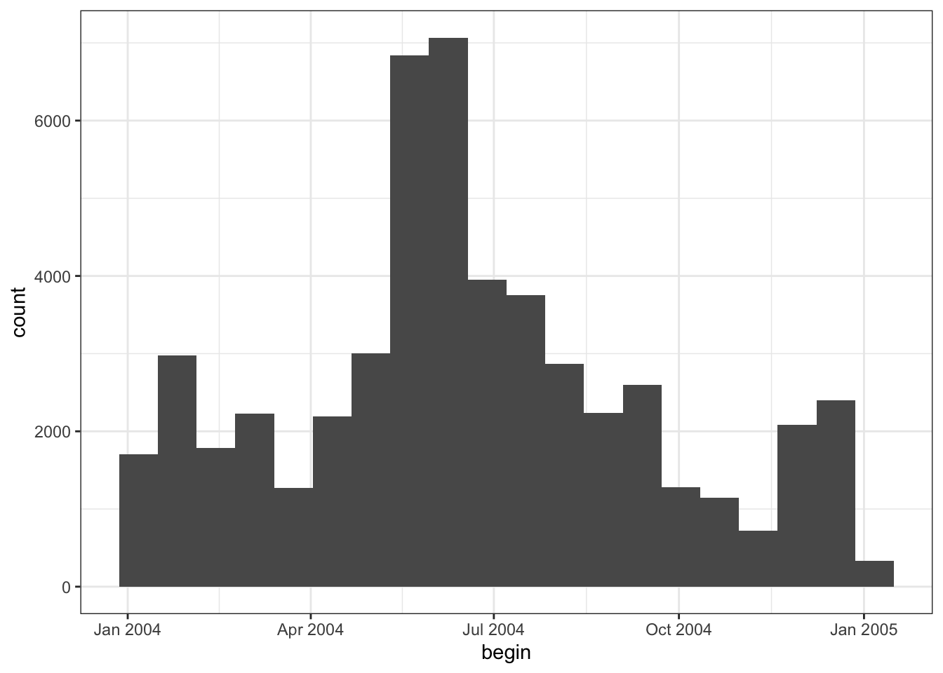

We can group by event type too.

library(ggplot2)
storm_sub %>%
  ggplot(aes(x = begin)) + 
  facet_wrap(~ type) + 
  geom_histogram(bins = 20) + 
  theme_bw() + 
  theme(axis.text.x.bottom = element_text(angle = 90))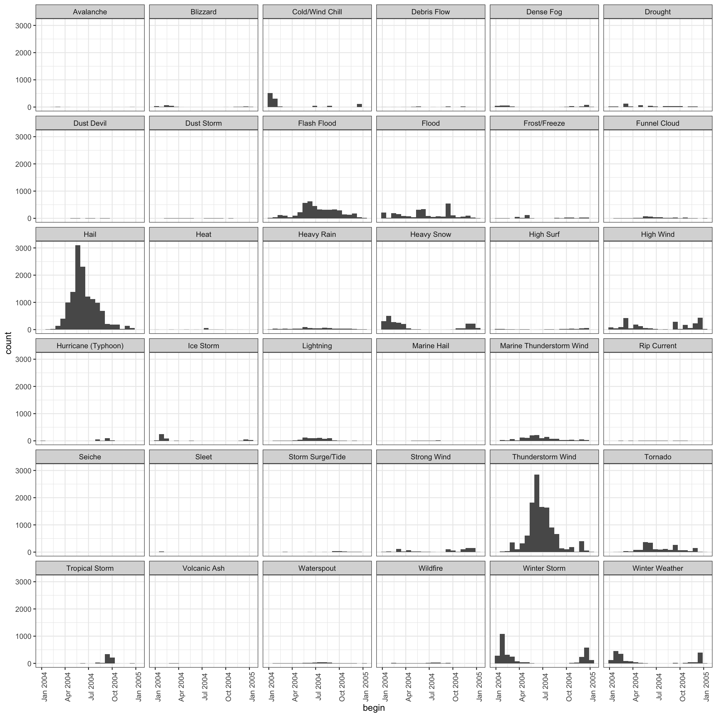

Scatterplots of Dates/Times

storm_sub %>%
  ggplot(aes(x = begin, y = deaths)) + 
  geom_point()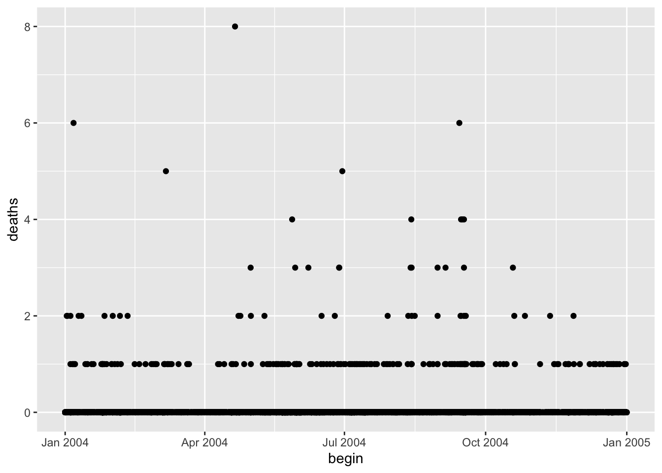

If we focus on a single month, the x-axis adapts.

storm_sub %>%
  filter(month(begin) == 6) %>%
  ggplot(aes(begin, deaths)) + 
  geom_point()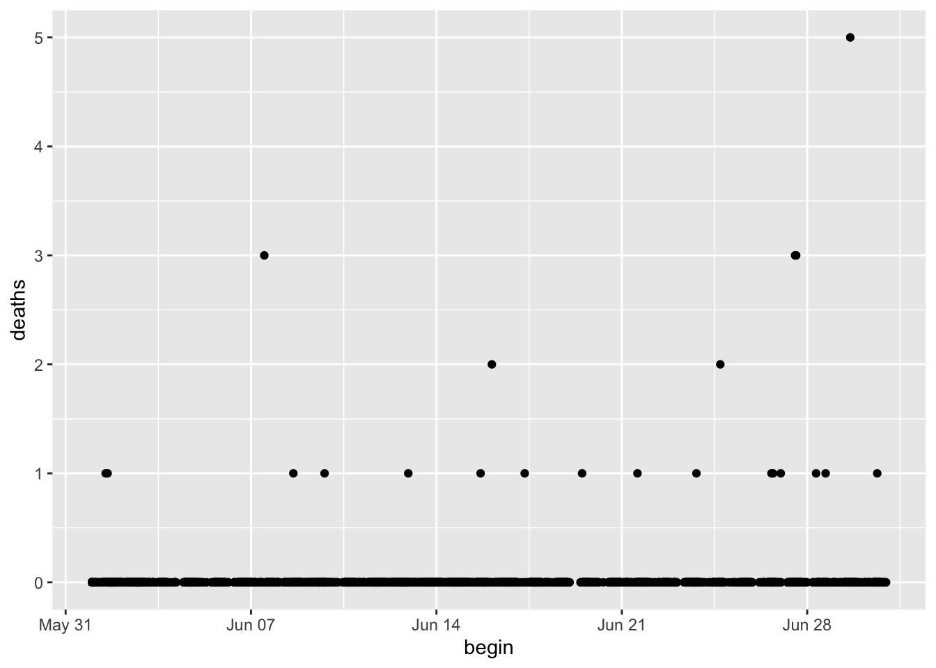

Similarly, we can focus on a single day.

storm_sub %>%
  filter(month(begin) == 6, day(begin) == 16) %>%
  ggplot(aes(begin, deaths)) + 
  geom_point()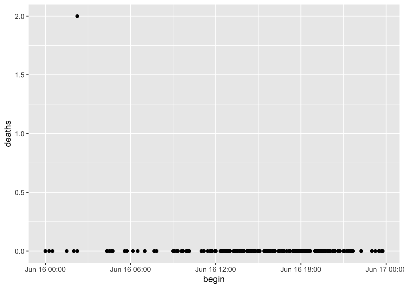

Summary

Dates and times have special classes in R that allow for numerical and statistical calculations
Dates use the Date class
Date-Times (and Times) use the POSIXct and POSIXlt class
Character strings can be coerced to Date/Time classes using the ymd() and ymd_hms() functions and friends.
The lubridate package is essential for manipulating date/time data
Both plot and ggplot “know” about dates and times and will handle axis labels appropriately.

Post-lecture materials

Final Questions

Here are some post-lecture questions to help you think about the material discussed.

Questions

What happens if you parse a string that contains invalid dates?

ymd(c("2010-10-10", "bananas"))

What does the tzone argument to today() do? Why is it important?

unclass(today())

[1] 19267

Use the appropriate lubridate function to parse each of the following dates:

d1 <- "January 1, 2010"
d2 <- "2015-Mar-07"
d3 <- "06-Jun-2017"
d4 <- c("August 19 (2015)", "July 1 (2015)")
d5 <- "12/30/14" # Dec 30, 20

Using the flights dataset, how does the distribution of flight times within a day change over the course of the year?
Compare dep_time, sched_dep_time and dep_delay. Are they consistent? Explain your findings.

Additional Resources

Tip

Pre-lecture materials

Read ahead

Acknowledgements

Learning objectives

Introduction

The lubridate package

Creating date/times

1. From a string

Alternate Formulations

2. From individual date-time components

3. From other types

Date-Times in R

From a string

POSIXct or the POSIXlt class

POSIXct

POSIXlt

Time Zones!

Operations on Dates and Times

Arithmetic

Leaps and Bounds

Extracting Elements of Dates/Times

Date Elements

Time Elements

Visualizing Dates

Reading in the Data

Histograms of Dates/Times

Scatterplots of Dates/Times

Summary

Post-lecture materials

Final Questions

Additional Resources

The `lubridate` package

`POSIXct` or the `POSIXlt` class

`POSIXct`

`POSIXlt`